Moiré Gravity and Cosmology — Alireza Parhizkar

The vacuum catastrophe is the largest numerical discrepancy in physics: the cosmological constant we observe is many orders of magnitude smaller than the one the theory expects. This paper does not fix it by making anything small. It builds a construction in which the small number is a difference between two large ones, and then asks what such a universe would have to look like.

The answer is unusually constrained. Almost nothing is put in by hand: the causal structure, the path integral and the requirement of diffeomorphism invariance do most of the choosing, and what comes out the other side is a single scalar field with a great deal to do.

Two worlds, and the fields that live on both

A universe with two geometries is not two universes unless nothing can cross between them.

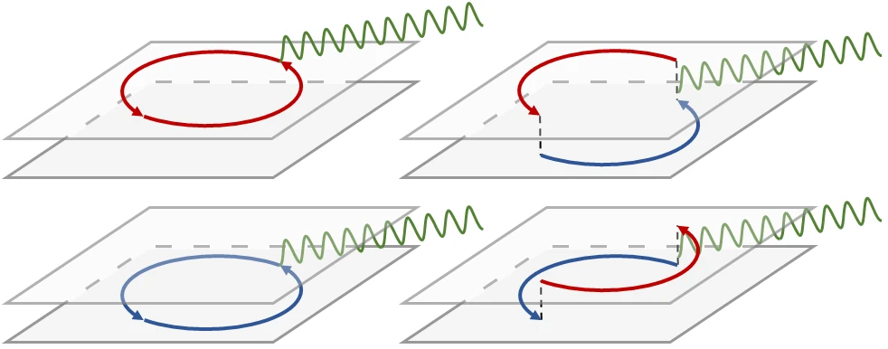
Write the action as : what lives only on the -world, what lives only on the -world, the cross terms, and — the interesting case — the amphibian fields that live on both. Without and the two worlds could not talk, and would simply be two separate theories.

For physicists

On a curved background the fundamental variables carry a fourth root of their own metric determinant, , which is what makes the measure diffeomorphism invariant. A cross term between the worlds then arrives with a crossbreed volume element:

Out of the bi-world construction, therefore, comes an inter-world vacuum energy density that couples to gravity as .

Eqs. (1)–(2) · equation numbers throughout are those of arXiv:2204.06574v2

A new scalar that only two metrics can have

With one metric, the only thing you can build out of its determinant is a volume. With two, you can build a number.

Terms in Einstein’s equations that describe vacuum energy are the ones proportional to the metric, and those come from terms in the action that depend on the metric only through its determinant. With a single metric there is exactly one such term, the four-volume. With two metrics there is a genuine scalar — the ratio of the two determinants — and any power of it can be used.

For physicists

Both determinants are tensor densities of the same weight, so the Jacobians cancel in the ratio and is a scalar under general coordinate transformations. If either metric is dynamical, a kinetic term for is expected — so it is a candidate for a field that describes the vacuum and relaxes it.

It is not only that. Writing the cross terms with a single volume element, appears multiplying inter-world fermion bilinears, gauge-field couplings and — Higgs-like in the first, axionic in the last, and modifying the chiral anomaly through .

Eq. (3)

Causality throws one degree of freedom away

Two metrics mean two sets of light cones, and a field that lives on both worlds would be able to tell them apart. That costs something.

A single metric can always be brought to Minkowski form at a point. Two cannot, in general, be brought there together — so a point has two futures and two pasts, and they need not agree. But an amphibian field feels both. Sketch the light cones from the commutators it obeys and you find the two structures must eventually be shared.

The argument that does the work is a counting one. Where the two causal structures disagree there is less accessible volume, and so exponentially fewer microstates. Summing over all pairs of metrics, the configurations that survive are the ones whose light cones coincide — which is to say the ones related by a conformal factor. That factor is exactly the scalar of the previous section.

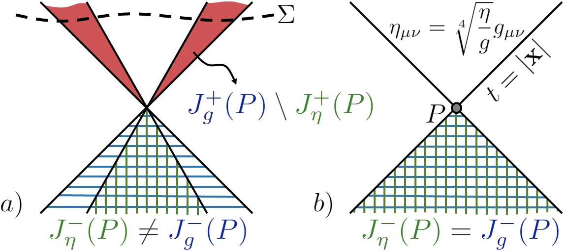
Two hatched regions showing the past of a point according to each of two metrics; in the first panel they disagree, in the second their light cones coincide. — **Two pasts, or one.** Horizontal hatching is the past of according to , vertical hatching according to . In (a) they do not match, and the region between them is effectively forbidden to excitations of an amphibian field. Configurations like (b), where the cones coincide, are favoured by an exponential factor of that region’s volume. Fig. 1 of the paper.

For physicists

The bi-metric path integral collapses to one metric and one scalar. This is the step that distinguishes the construction from bimetric and massive gravity: the reduction is forced rather than imposed, gravity stays massless, and in the vacuum limit the model is two massless gravity theories and therefore ghost-free.

Eq. (5)

Integrate it out and Starobinsky appears

The scalar was not put in to drive inflation. It drives inflation anyway.

Substituting the conformal relation into two Einstein–Hilbert actions joined by their shared volume element gives one action in one metric and one scalar. Solve for the scalar at the saddle point and what is left is the Starobinsky action — the inflation model, arriving here from a bi-world construction rather than from quantum corrections.

For physicists

From

the classical field equations read : each world sees the other only as an addition to its own cosmological constant. Substituting and taking the saddle point at ,

Eqs. (6)–(9)

Or let it roll

Out of equilibrium, the two worlds carry an enormous vacuum energy. In equilibrium they carry none. Friction takes them from one to the other.

Conformally rescaling to a minimally coupled theory and taking the usual homogeneous, isotropic ansatz, the scalar becomes a single particle rolling on a potential — a Mexican hat, with the equilibrium at the bottom of the brim. The Hubble rate is not free to do as it likes: it can only decrease, and it decreases exactly when the scalar is moving.

So the history is a shape rather than a fit. Two worlds start out of step; the scalar rolls, overshoots and oscillates about equilibrium; and every oscillation costs the expansion rate something it cannot get back. Where the roll is slow, the expansion sits still — an inflationary stretch, arriving as a feature of the descent rather than as an assumption.

φ at the start 1.50 k H at the start: —_P

Fig. 2, integrated here. Equations (11) and (12) with the paper’s own numbers — , , starting at 1.5. The Hubble rate is never integrated: it is fixed at each instant by the Friedmann constraint, and at that gives , the the paper’s caption quotes. then oscillates about 1 and falls monotonically. Where moves slowly, is flat.

For physicists

The conservative force in the equation for vanishes at ; the potential is a Mexican hat, except at where the crown is lifted to infinity. The expansion obeys

so for every the Hubble parameter is ever-decreasing up to equilibrium, while the constraint ties a non-equilibrium to a large vacuum energy density. Relaxation, not tuning.

Eqs. (10)–(14)

Why the two constants must oppose each other

The equilibrium has to be stable, and that alone fixes a sign.

Two similar worlds have similar constants, so the natural scale for each is the Planck scale. The inter-world vacuum is built from the same fields and the same processes as the intra-world one — for every vacuum loop inside one world there is a counterpart that passes through both — so its magnitude is fixed too. What is left to decide is a sign, and stability of the equilibrium decides it: the inter-world constant must oppose the intra-world ones.

Diagrams of external gravitons coupling to vacuum loops: on the left loops within one world, on the right loops that pass through both. — **Loops inside one world, and loops through both.** External gravitons (wiggly) coupling to intra-world vacuum loops on the left and inter-world ones on the right. For each loop in a single world there is a counterpart passing through both, which is the counting that sets the magnitude. Fig. 3 of the paper.

What would falsify it

The axionic term does not stay quiet. Integrated out, it modulates the scalar’s potential in an oscillatory way near the extrema — a trace the paper expects early-universe observations could look for. That is the offered handle, and it is offered as a handle rather than a prediction.

The rest of the distinction from bimetric and massive gravity is structural: the metrics couple to each other and to matter differently; there are two worlds here rather than two metrics, with matter fields whose effects are meant to be observable; the scalar is emergent and inherently geometric; and gravity stays massless throughout.

The construction this paper develops was set out first in Strained Bilayer Graphene, Emergent Energy Scales, and Moiré Gravity, where it arrives out of a sheet of graphene.