Zero-Flux Localization — Alireza Parhizkar

A flat band is a way of saying that an electron will not move, however hard you push it: its energy does not depend on its momentum, so there is no direction downhill to go. The oldest example is a uniform magnetic field, where the electron simply goes round in a circle and comes back to where it started. What makes that work is that the field never cancels.

This Letter asks what is left when it does. The answer has three parts, and the third is the one that carries: a field with zero total flux cannot flatten a band; adding a spin field that carries no flux of its own restores it exactly; and once the plane is tiled and rolled into a torus, that only works at particular field strengths — the magic values, which turn out to be flux quantisation through a single tile.

A field that never cancels

Put an electron in a uniform magnetic field and its energy levels stop depending on its momentum altogether. That is Landau quantisation, and is the statement that the electron is stuck where it is.

Make the field lumpy and momentum is no longer a good quantum number — the translational invariance is gone. But the question of whether there are still highly degenerate, dispersionless levels survives, and it has a known answer whenever the total flux through the system is not zero: if , then at least modes share an energy. A flat band.

For physicists

A relativistic electron in the plane, and its square, which is the same field seen by a quadratic dispersion:

Apart from the Zeeman term, is a massive electron of mass in the same field. Everything below is done for and inherited by , because the two share their zero modes: if then .

Eqs. (1)–(2) · equation numbers throughout are those of arXiv:2409.05942v1

What happens when it does

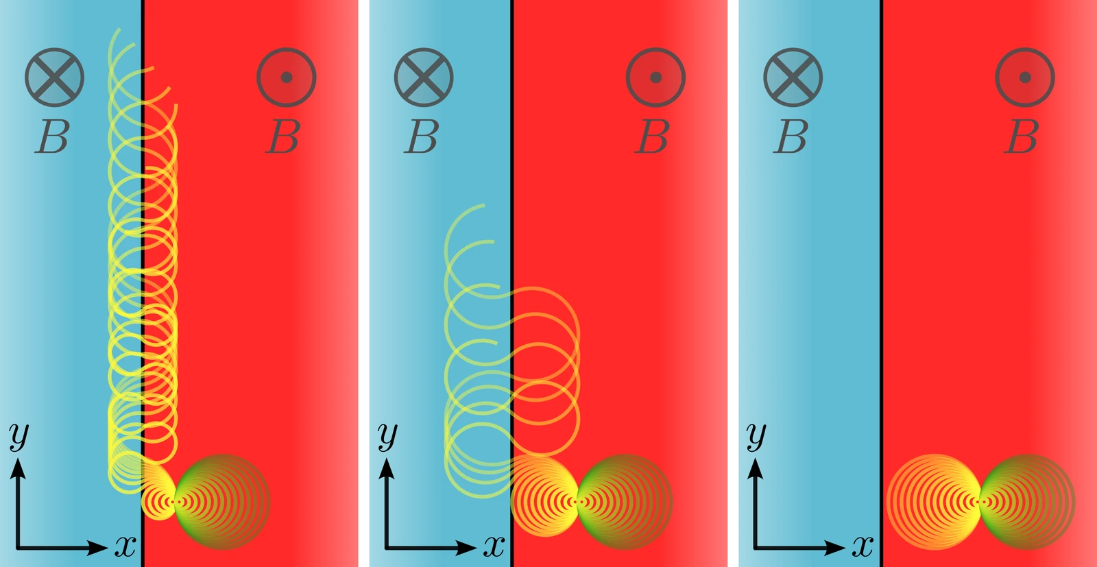
Take the simplest field that adds up to nothing: pointing one way for and the other way for , with the same strength on both sides. Classically the particle still goes in circles — but the two sides turn it opposite ways, so a particle that reaches the dividing line has to reverse its handedness to carry on. It does not close its orbit. It walks along the line.

B out of the page B into the page

One field

A uniform field, and the orbit closes. The particle comes back to where it started, over and over: the return probability is one, and that is localization, classically.

Two fields, adding to nothing

Now reverse the field across the vertical line. Every time the particle crosses, it must turn the other way. Two half-circles of opposite handedness do not close — they staircase along the boundary, and the particle leaves.

Which way it drifts depends on the sign of the charge. That it drifts at all does not.

How close you start decides everything

Start far enough out and the orbit never touches the line: that particle is as trapped as it was in the uniform field. Start nearer and it escapes, and the nearer it starts the faster it goes. There is no distance at which the escaping trajectories stop existing.

That is the whole classical obstruction. And by the path integral it is a quantum obstruction too: if a trajectory to infinity exists, there is amplitude for it.

Three panels showing classical trajectories of a charged particle in a magnetic field that flips direction at x = 0; the closer the particle starts to the boundary, the further it travels along it. — **Fig. 1.** Blue and red are the two field directions; the particle’s starting point moves closer to the boundary from right to left. In a homogeneous field the return probability is one; in this one, unbounded trajectories always exist. Fig. 1 of the Letter.

The quantum version says the same thing

Keep the translational symmetry along and the Schrödinger problem collapses to one dimension: a particle in the potential . Drop the absolute value and it is the harmonic oscillator, the same at every — Landau quantisation, flat. Keep it, and the shape of the potential depends on , so the energy does too.

Two limits pin it down. At the potential is a single harmonic well and the ground state sits at . At large there are two wells so far apart that they no longer talk, and the ground state is again. Between them the energy has to dip. Drag below and watch where it does.

k_y E = — ∂E/∂k_y = —

Fig. 2, solved here. The ground state of on a grid, for every on the axis. Yellow is the potential, blue the ground state, black the band. The group velocity is negative before the minimum and positive after it — so momenta below zero are forbidden, and yet downward propagation still exists.

The band is not flat, and the reason it is not flat is the classical one written in quantum mechanics: the escape has become a group velocity.

Where it actually breaks

The obstruction is clearest for the relativistic electron, where the zero modes can be written down. The two spinor components decouple, and each is any holomorphic function of dressed by a scalar potential fixed by the field.

For physicists

Poisson always has a solution, so these always exist. Which of them is normalizable is what the field decides: for only is bounded, for only .

Eqs. (6)–(7)

Now put the two half-planes together. On the right only the upper component survives; on the left only the lower one. The only candidate left is a spinor that is one thing on one side and the other thing on the other — and that spinor is perfectly normalizable but it jumps across the line, so it does not solve the equation. Integrate the Dirac operator across an infinitesimal interval and the derivative hands back exactly that jump.

For physicists

Normalizable, discontinuous, and therefore not a solution. No zero mode exists.

Eqs. (10)–(11)

A patch that costs no flux

A discontinuity in the wavefunction is repaired by a singular potential sitting exactly where the jump is. Put a delta function on the dividing line — not in the electromagnetic field, but in a spin field, one that multiplies and so acts on the two components with opposite signs. That is precisely what is needed to sew a spin-up half onto a spin-down half.

For physicists

With in place there are infinitely many zero modes, and the count changes character. Before, the number of normalizable zero modes was set by the total flux, which here is zero. Now it is set by the total absolute flux, — while itself carries no flux at all, so the system as a whole is still flux-less.

Eq. (12)

The delta function is a convenience, not the mechanism. Replace the line by a ribbon of finite width with no magnetic field in it, and the spin can be turned from down to up gradually as the electron crosses; the zero mode survives, written out explicitly, with a smooth instead of a singular one.

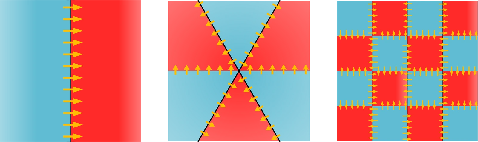
Nothing about the construction cares that there was one line. Cut the plane up any way at all — let be where the field points up, where it points down, and zero on the cuts. Then the patching field is just : deltas living on the dividing lines, pointing away from the downward regions. Every one of these configurations has zero modes.

Three ways of dividing a surface into regions of upward and downward magnetic field: one straight line, three lines through a point, and a checkerboard of square tiles; yellow arrows sit on every dividing line. — **One line, three lines, a checkerboard.** Any of them, and checkerboard: the yellow arrows are , sitting on the cuts and pointing away from the downward regions. All of these have infinitely many zero modes, because adding a dividing line never leaves the patching recipe. Fig. 4 of the Letter.

Why this is bilayer graphene

Give the construction a second layer, carrying the opposite field. Now the jump at the line has four components rather than two, and there is more than one way to repair it. The obvious way patches each layer to itself. The other way patches across the layers — the upper component of one against a component of the other.

Two stacked planes with opposite magnetic fields, patched within each layer along the dividing line. — **Two ways to sew it.** Above, each layer is patched to itself. Below, the patch runs between the layers. Only the second leaves a gauge field that fails to commute with itself from point to point — and that, not the number of layers, is what makes it non-Abelian. From the thesis defence; cf. Fig. 3 of the Letter.

The same two planes patched across the layers instead, the patching field spanning the gap between them. — **Two ways to sew it.** Above, each layer is patched to itself. Below, the patch runs between the layers. Only the second leaves a gauge field that fails to commute with itself from point to point — and that, not the number of layers, is what makes it non-Abelian. From the thesis defence; cf. Fig. 3 of the Letter.

For physicists

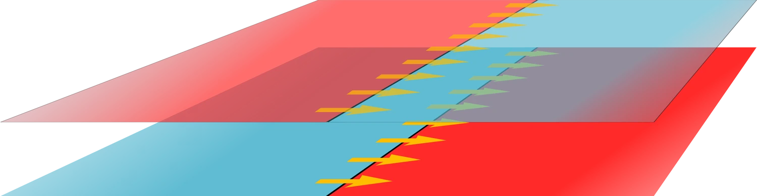
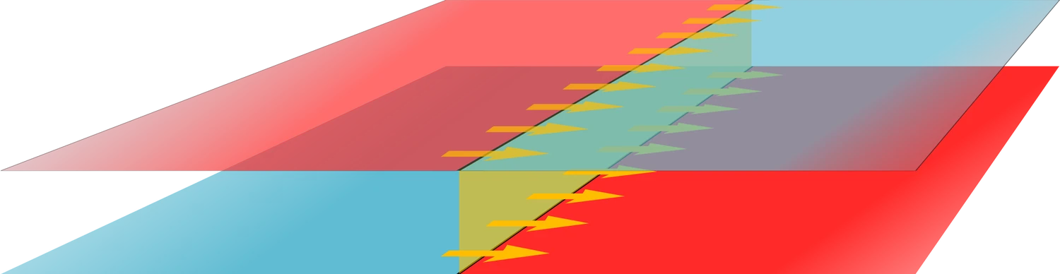
The interlayer patch enters as a spin field proportional to . The overall gauge field does not commute with itself at every point, which is the whole content of the word non-Abelian here. Compare this action with the continuum theory of a mutually deformed — twisted or strained — bilayer: it is the same theory.

Eqs. (14), (17)–(18)

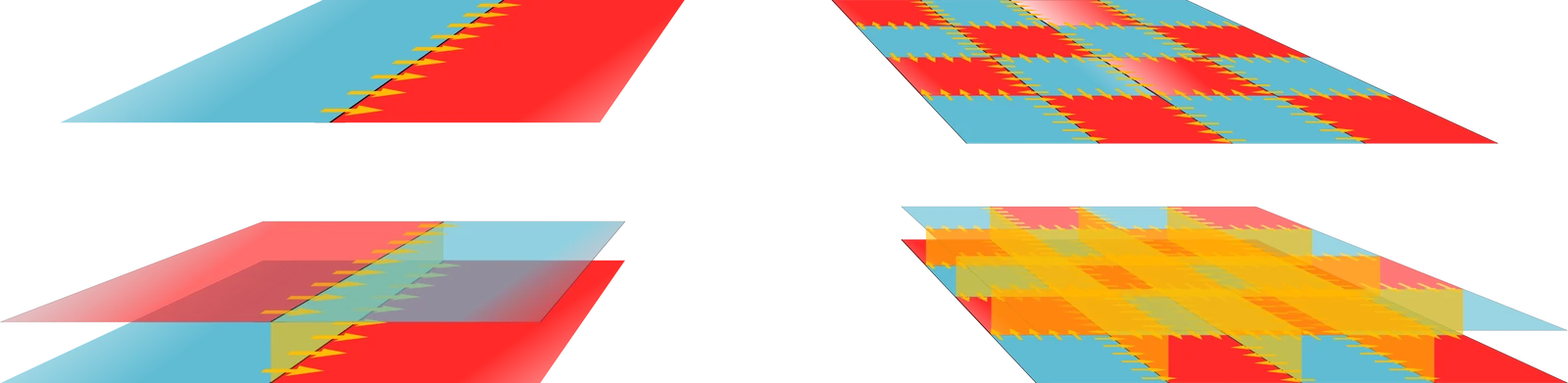
On the left, one dividing line promoted to a bilayer with non-Abelian fields; on the right, a tiled surface and its bilayer counterpart. — **And it does not stop at one line.** Left, the single-line example as a bilayer. Right, the same promotion applied to a whole tiled surface — which is where the twisted bilayer is. Fig. 3 of the Letter.

This is the sense in which a toy model earns its keep. The half-plane example was chosen because it can be solved on paper; what comes out of it is the structure that twisted bilayer graphene has anyway.

Roll it up, and only certain fields work

Two more surfaces, and they behave differently from each other. On a cylinder — alternating strips, periodic in one direction — the zero modes can be written down in closed form, and the gauge choice that makes them manifestly normalizable also shows that the problem cannot be reduced to one dimension. Zero-flux localization is two-dimensional by nature.

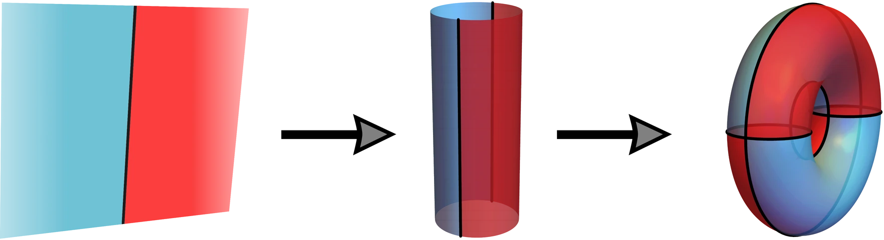
A flat sheet divided into red and blue magnetic regions, then rolled into a cylinder, then closed into a torus. — **The plane, the cylinder, the torus.** On the first two the flat band can always be rectified. On the torus it cannot. From the thesis defence.

On the torus, periodic in both directions, the zero modes are theta functions and the wavefunction has to come back to itself after a full turn. It does not, generally: going once round leaves two stray factors behind, and only one class of theta function cancels them. Cancelling them is a condition on the field strength.

flux through one tile 1.00 after one turn: × 1.00

Coming back to itself. The toroidal zero mode evaluated over two turns. The dashed curve is the first turn moved along by one period — where the solid curve should land. The two agree only when the flux through a single tile is a whole number of flux quanta; between those values the wavefunction is not periodic and there is no state.

For physicists

Matching the quasi-periodicity of against the Gaussian requires and together, that is . Raising the theta function to the th power gives another zero mode, so the criterion relaxes to

The periodicity is set by the dividing lines, which cut the surface into magnetic tiles; the condition for localization is that the flux through one tile be an integer number of flux quanta. These are the magic values, and they agree with the topological criterion argued from the index theorem in the earlier paper.

Eqs. (20)–(23)

There is a correction with a real consequence. The patching field does not sit outside the count: where it coexists with it adds effective flux to each tile, and so it moves the magic values. In twisted bilayer graphene, ignoring it gives ; putting the effective flux back gives .

0.586 is the first magic angle of the chiral model. The Letter arrives at it by putting the patching field’s own flux back into the count.

What it opens

Exact solutions are worth having for what can be built on them. Two things are named at the end of the Letter. The first is a class of fractional quantum Hall states with no net flux: the flat bands here come with a spin texture, and Laughlin-like wavefunctions can be written from the elliptic-function spinors — which are not the ones in the textbook. The second is that flat-band localization need not be imposed from outside. Nearly dispersionless electrons can develop the periodic texture themselves, through a phase transition, in the charge channel, the superconducting channel, or the spin channel depending on which one the energetics prefers.